Heteroskedasticity of unknown form (González-Coya and Perron, 2024)
Source:vignettes/heteroskedasticity.Rmd
heteroskedasticity.RmdThe idea
When \(\mathrm{Var}(u_t) = v_t\) varies across observations, weighted least squares with weights \(1/v_t\) is efficient. The variances are unknown and their functional form is rarely known. The approach of the 2024 paper:
- run OLS and form \(r_t = \log \max(\hat
u_t^2, \delta^2)\), where the floor \(\delta = 0.1\) (
delta, in the units of \(y\)) avoids \(\log 0\); - regress \(r_t\) on a dictionary of candidate covariates \(z_t\) by an adaptive Lasso. A ridge regression gives weights \(|\hat\gamma^{ridge}_j|^{-\psi}\), and the penalty \(\lambda\) and the exponent \(\psi \in \{0, 0.25, 0.5, 0.75, 1, 2\}\) are chosen jointly by 10-fold cross-validation, with the same folds for every \(\psi\);
- use \(\exp(\hat r_t)\) as the variances in weighted least squares.
Because the skedastic model is an approximation, the variance of \(\hat\beta\) is a sandwich (eq. 6) with a bias correction for the estimated weights (eq. 8). Confidence intervals therefore remain valid when the model for \(v_t\) is wrong.
An example
het <- simulate_hetero(200, skedastic = "log2", seed = 10)
fit <- lasso_fgls(y ~ x, data = het, seed = 1)
summary(fit)
#>
#> Call:
#> lasso_fgls(formula = y ~ x, data = het, seed = 1)
#>
#> Method:                 FGLS (hetero)
#> Covariance:             robust
#> Observations:           200
#> Inference:              normal
#> Skedastic fit:          lasso
#> Selected z:             log(x)^2, cos(x), cos(2x)
#> Lasso psi, lambda:      2, 0.01405 (glmnet scale; 2.809 in GP24 eq. 4)
#> df_hat:                 4
#> Variance ratio max/min: 118
#>
#> Coefficients:
#>             Estimate Std. Error z value Pr(>|z|)
#> (Intercept)  0.97277    0.07472   13.02   <2e-16 ***
#> x            1.00314    0.05128   19.56   <2e-16 ***
#> ---
#> Signif. codes:  0 '***' 0.001 '**' 0.01 '*' 0.05 '.' 0.1 ' ' 1
#>
#> Notes:
#> [1] Covariance: GP24 eqs. (6)+(8), sandwich with bias correction.
The summary reports the selected covariates, \(\psi\), \(\lambda\) and the degrees of freedom of the skedastic fit used in the bias correction (the number of non-zero coefficients, intercept included).
fit$skedastic$coefficients
#> (Intercept)           x         x^2      log(x)    log(x)^2      cos(x)
#>  -4.0246234   0.0000000   0.0000000   0.0000000   0.8343119  -3.2904036
#>     cos(2x)
#>  -1.6605147
plot(fit, which = 4)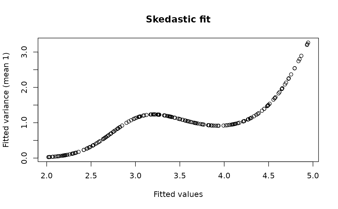
Candidate covariates
z = "auto" (the default) builds \(x, x^2, \log x, (\log x)^2, \cos x,
\cos 2x\) from every non-constant regressor
(make_dictionary()), which includes the specification of
the paper’s simulations. Dummies are passed through untransformed. You
can pass names of regressors, a one-sided formula, or a matrix,
including covariates that are not regressors:
het2 <- simulate_hetero(200, skedastic = "x2", n_extra = 3, seed = 11)
fit2 <- lasso_fgls(y ~ x, data = het2, z = ~ x + I(x^2) + w1 + w2 + w3, seed = 1)
fit2$skedastic$selected
#> [1] "x"  "w1" "w2" "w3"
The Lasso copes with many candidates, even more than observations. In the paper’s robustness designs with about 60 candidates it loses little against OLS when the true driver is absent, and gains when it, or a correlated proxy, is present.
No loss under homoskedasticity
If nothing is selected, the weights are constant and FGLS equals OLS:
hom <- simulate_hetero(200, skedastic = "homoskedastic", seed = 12)
fit_h <- lasso_fgls(y ~ x, data = hom, seed = 1)
fit_h$skedastic$selected
#> character(0)
all.equal(coef(fit_h), coef(lm(y ~ x, data = hom)))
#> [1] TRUE
Alternatives and benchmarks
-
hetero = "wls_s1"and"wls_s2"are the parametric skedastic functions of Romano and Wolf (2017), \(\exp(c + \gamma'\log z)\) and \(\exp(c + \gamma'z)\), with their HC3-type variance (eq. 7); -
hetero = "svr"uses support vector regression (requires ‘e1071’); -
hetero = "known"withvariancegives GLS with known variances, the infeasible benchmark; -
hetero = "none"is OLS with HC3 standard errors.
sapply(
  list(
    OLS = lasso_fgls(y ~ x, data = het, hetero = "none"),
    `WLS-S1` = lasso_fgls(y ~ x, data = het, hetero = "wls_s1", z = "x"),
    Lasso = fit,
    GLS = lasso_fgls(y ~ x, data = het, hetero = "known", variance = attr(het, "info")$v)
  ),
  function(f) sqrt(vcov(f)[2, 2])
)
#>        OLS     WLS-S1      Lasso        GLS
#> 0.08617975 0.05456243 0.05127991 0.05580638
Weights and robustness options
weight_diagnostics() summarizes how concentrated the
weights are; extreme weights trigger a warning.
weight_clip = c(0.01, 0.99) winsorizes the fitted
log-variances, and fgls_control(delta_scale = TRUE) makes
the floor proportional to the residual standard deviation.
weight_diagnostics(fit)
#>       variance_ratio    effective_n_share top1pct_weight_share
#>          118.4843042            0.2082983            0.1147883